
Stable Player Impact (SPI) is a plus-minus impact metric that I have been thinking about building out for a while. Recently I got it to a point where I am ready to release it publicly. (Note that I reserve the right to tweak it and improve it without notice! I make no apologies!)
Stable Player Impact has very few original ideas. Instead I borrowed liberally from other people’s ideas, most of whom I consider friends or at the very least acquaintances. The biggest inspiration for and reason why I made SPI is Player Impact Plus-Minus (PIPM). In fact, when I was first building it out and telling others about it, I would simply call it “knockoff PIPM.” PIPM is the creation of Jacob Goldstein (with an assist from Nathan Walker on the development of the luck-adjustment for lineup data).
At the start of the 2020-21 season, fortunately for Jacob, but unfortunately for those of us who liked using PIPM in the public domain, he was hired by the Washington Wizards and PIPM went dark. Since then, I’ve wanted to recreate the metric for my own personal use, but I didn’t want to just do exactly what Jacob did, because well, that doesn’t feel very inspired and I thought there were some additional tweaks I could make to the process to maybe improve it. In broad strokes, however, the two metrics could be considered siblings or at the very least first cousins. They have very similar DNA.
Creating Bayesian Luck-Adjusted / Stabilized On-Off Data
The core insight of PIPM was that on-off data could be “luck adjusted” using mean regression for different components of the four factors. This was accomplished using a leave one out regression using one game to predict the Offensive or Defensive Rating of each team for the other 81 games in a season across a number of seasons. I decided to take a similar but different approach. My approach considers the sample of possessions in both the on sample and the off sample for both the player’s team and their opponent to mean regress each of the individual components of the four factors using a method very similar to the “padding method” popularized by Kostya Medvedovsky, the creator of DARKO. I found the padding values used by using empirical Bayes, rather than differential evolution like Kostya used for the padding method on individual box score stats. I then plug these Bayesian, stabilized four factor component values into a formula developed via regression on data from 1997 to 2022 that has a .95 r-squared with player-on-the-floor Offensive Rating (plot of actual versus predicted ORtg below):
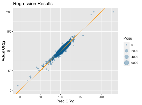
Here are the weights for predicting Offensive or Opponent Offensive Rating based on this regression:
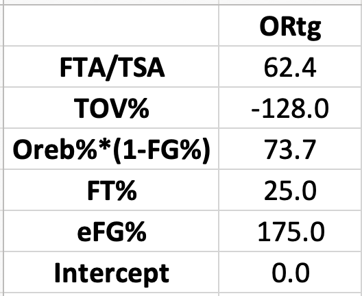
TOV% here is TOV/(FGA+.44*FTA+TOV) and FTA/TSA is .44*free throw attempts divided by true shot attempts (FGA+.44*FTA).
Creating the Box Score Component
SPI was created using a regression against 26 year RAPM, provided to the public domain by former Suns analyst Jerry Engelmann, while PIPM was created using a 15 year RAPM basis (also via Jerry). Like PIPM, there is a box score component to SPI. It includes the same per-possession stats and Games Started % squared term as PIPM, although the weights are not exactly the same as the RAPM basis is different and I use per 100 possessions, rather than per 75 possession numbers. I also used 10×10 cross-validation for both the offensive and defensive box-score regressions to minimize overfitting. The r-squared on these heavily cross-validated values is .72 for Box O-SPI and .59 for Box D-SPI.
The box-score coefficients for SPI are as follows:
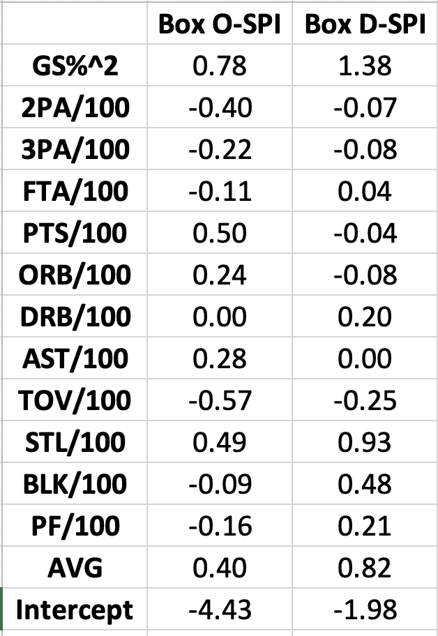
Where AVG is the team’s overall Bayesian, stabilized luck-adjusted ORTG or DRTG minus league average and multiplied by a player’s percent minutes played and GS%^2 is percent of Games Started squared.
Creating Stable Player Impact
The box-score portion from above is coupled with the aforementioned Bayesian luck adjusted on-off data for each player using the following equation:
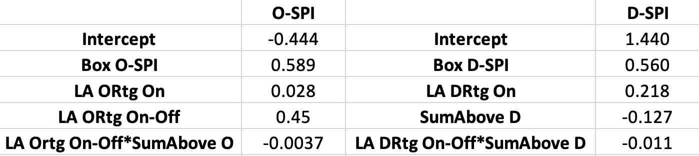
LA ORtg and DRtg On are the Bayesian, stabilized luck adjusted values for the team or opponent offensive rating from when the player is on the floor relative to the league average value for luck adjusted efficiency. The On-Off component is those On values with the same values calculated for when the player is off the floor subtracted out. Finally the “SumAbove” component is an idea borrowed from Ben Taylor‘s Augmented Plus-Minus metric (AuPM). I’ll let Ben explain it:
I played with the relationship between a player’s on/off and his teammates, and while many made minor improvements, the largest came from simply summing the difference of the 1000 MP teammates ahead of a player. For instance, take the following group of teammates:
Player A = 2.0
Player B = 5.0
Player C = 6.0
Player A’s “summed above” value would be the difference between himself and B plus the difference between himself and C, or 7.0.
https://thinkingbasketball.net/2017/09/18/augmented-plus-minus-evaluating-old-pm-data/
I made a slight tweak and used players who had played 25% of team possessions, rather than 1,000 minutes played, as the comparison teammates for the player for whom we are calculating SPI and obviously we are using luck adjusted on-off data rather than raw data and have it split out for offense and defense rather than using Net On-Off like AuPM does.
These coefficients for SPI were also produced using regression with 10×10 cross validation and the r-squared for O-SPI to 26 year O-RAPM is .80 and for D-SPI to 26 year D-RAPM is .74.
Each component of O-SPI and D-SPI is also stabilized heavily. The box-score values are stabilized using the padding method values here, only regressed toward league average rather than the specific values Kostya shows which were essentially the averages over the time of the sample he used to find the right padding value. The on-off components are mean regressed using the amount of possessions that best minimized the error between year n+1 values and the season considered. This is all necessary because the spread or variance in these values is much larger in a single season than in the 26 year sample, for obvious sample size reasons.
The last aspect of SPI is a team adjustment in the same way as the original version of Box Plus-Minus (and the same adjustment I used in calculating the team adjusted for my version of WNBA “BPM”). These adjustments are more impactful very early in the season when the spread of the metric is very compressed (though I try to reduce this some by mean regressing team level opponent-adjusted performance early in the season), but they become very small as the season progresses.
Wins Created
SPI can be translated into Wins numbers by using the Wins Created method that Nathan Walker developed for any per-100 impact style metric, which goes as follows:
Team Games*(norm.dist(SPI*(% of team minutes played),0,12.5,1)-0.5+0.5*.2*(% of team minutes played))
That looks like a lot, but the logic of it is fairly simple:
SPI*(% of team possessions played) is a player’s contribution to the scoring margin for the team over the whole year, and the normal distribution can be used to estimate a player’s win%, using a standard deviation of 12.5, with the mean of 0. Then we back out an average winning percentage (-0.5) to get the player’s impact to an average team. Then we add back in the impact that an average player would have had in the same number of minutes as the player played (0.5*0.2*(% of team possessions played)) to finally arrive at the number of wins this player could have been expected to add to an average team. These win totals should sum very close to 1230 wins for a normal 82 game season.
Results!
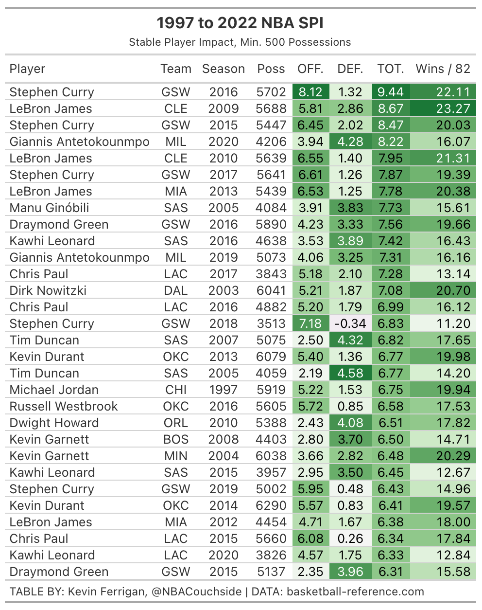
Here are the top 30 seasons in Stable Player Impact of the play-by-play era (1996-97 to 2021-22 seasons):
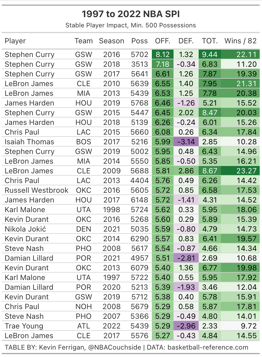
These are the top offensive SPI seasons in the play-by-play era:
Lastly, we have the top defensive SPI seasons of the last 26 years:

In the next few days, my aim is to have all of the last 26 years of SPI seasons up on a separate web page on this site, as well as the most up-to-date data for the 2022-23 season on its own page. In the meantime, here’s a link to a Google Sheet with the 1997 to 2022 data!
Thanks for reading!
